Quantitative equity models rarely fail because of faulty arithmetic. They fail because the assumptions that support the numbers are difficult to reconcile with reality. This usually means the assumptions about market behavior have not been sufficiently tested. When those assumptions prove untenable, the precision of the model’s output offers little protection.
Part I set out the elements of a buy-side model; viz. return on invested capital, growth, reinvestment, margins, cost of capital, and terminal assumptions. Those variables determine intrinsic value in any long-horizon framework. But each one is a summary of assumptions. ROIC reflects beliefs about competitive advantage and capital discipline. The growth rate reflects assumptions about market structure and response. Margins imply views on pricing power and cost behavior. Even the cost of capital is a statement about perceived risk, not a mechanical output. The numbers look objective. The judgments beneath them are not.
The purpose of Part II is to make those judgments explicit. It examines how qualitative factors shape the quantitative inputs already in the model, and why those factors deserve as much scrutiny as the numbers they produce. Each metric is paired with the underlying qualitative forces that influence its level and durability, and with examples that illustrate how small shifts in judgment can materially alter modeled value.
2. ROIC and Competitive Advantage: When Returns Are Earned vs. When They Are Assumed
2.1 The Qualitative Drivers of Sustainable ROIC
Sustainably high returns on invested capital rarely emerge by accident. Very often, they will result where there is limited competition or good opportunity for incremental capital to be deployed. Barriers to entry matter most when they are structural rather than transient. Structural barriers, such as regulatory licenses, network effects, or high asset specificity, limit the ability of new entrants to replicate the business economics. Transient advantages, by contrast, such as a temporary cost lead or early-mover scale, often invite imitation and erode over time.
Pricing power and customer captivity are closely related. Businesses that can raise prices without materially impairing volume usually are benefiting because of high switching costs, embedded workflows, or well-differentiated offerings. Where customers are price-sensitive and alternatives are readily available, high historical ROIC is more likely to reflect favorable conditions than durable advantage. Capital intensity also plays a role. Asset-heavy businesses with specialized assets may deter entry, but they also face higher reinvestment needs and greater downside risk if demand weakens. Asset-light models can scale rapidly, but often attract competition more quickly.
Finally, organizational discipline in capital allocation is critical. Even businesses with strong competitive positions can destroy value if management allocates capital indiscriminately, overpaying for acquisitions, venturing into low-return projects, or pursuing growth for its own sake. These qualitative factors help explain why historical ROIC is evidence of past success, not proof of future returns. Forward ROIC, by contrast, is a hypothesis about how competitive dynamics, capital allocation, and industry structure will evolve.
2.2 Common Analytical Errors in ROIC Assumptions
Several recurring mistakes undermine ROIC-based analysis. One is treating peak-cycle ROIC as normalized, particularly in cyclical industries where margins and utilization temporarily inflate returns. Another is assuming that scale automatically preserves returns. In many industries, growth attracts competitors, reduces pricing, or raises regulatory scrutiny. A third error is ignoring the distinction between legacy capital and incremental capital. Returns earned on assets deployed years ago may have little bearing on what new investments can earn under current conditions.
2.3 Illustrative Example: ROIC as a Judgment Call
Consider a regulated infrastructure business, supported by limited competition and favorable regulatory treatment, that has earned consistently high ROIC over the past decade, Suppose, however, that the regulatory framework changes, allowing greater rate scrutiny or encouraging new entrants through revised access rules. Reported ROIC may remain elevated in the near term, reflecting the productivity of legacy assets and contracts. A reasonable analyst, however, would likely normalize forward ROIC downward. The key judgment is not that returns will collapse overnight, but that incremental capital will earn less than historical capital.
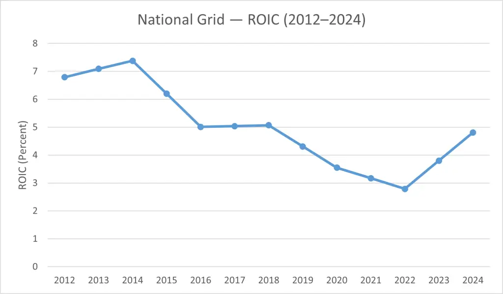
Case Study: National Grid
For many years, National Grid enjoyed sustainably high returns on invested capital. Operating regulated electricity and gas transmission networks in the UK and the northeastern United States, the company benefited from powerful structural barriers that included exclusive licenses, asset specificity, and non-discretionary demand. Customers could not readily switch providers, and regulators explicitly allowed the recovery of invested capital plus a fair return. In this setting, high ROIC was earned rather than assumed.
These returns were not the product of transient advantages or cyclical conditions. They reflected a stable institutional framework in which incremental capital deployed into the regulated asset base reliably earned returns above the cost of capital. Historical ROIC therefore captured genuine economic strength.
The analytical challenge emerged gradually as regulatory frameworks evolved. In the UK, regulators began to tighten allowed returns, increase efficiency requirements, and apply greater scrutiny to new capital spending. Crucially, these changes did not immediately reduce reported ROIC. Legacy assets, approved under earlier regulatory regimes, continued to earn their contracted returns, keeping headline metrics elevated even as the economics of new investment shifted. But after a while, the effect of the regulatory shift became apparent.
In Britain, implementation of the RIIO (Revenue = Incentives + Innovation + Outputs) framework took off in 2013. So that by the end of 2014, legacy ROIC momentum was exhausted. Thereafter, ROIC fell and continued to fall for eight years. The decline ceased in 2022. It had taken almost a decade for National Grid to adjust to the new regime. The business had not become operationally weaker; but the terms under which new capital could earn returns had changed.
3. Revenue Growth and Market Structure: Where Growth Comes from and What It Costs
3.1 Qualitative Sources of Growth
In a buy-side framework, all revenue growth is not equal; some types are decidedly preferable to others as the following distinctions will make clear. The first distinction to be made is between market expansion and share gains. Growth driven by population increase, rising penetration of a product category, or favorable macro demand, will be less adversarial. Growth driven by gains in market share, by contrast, is inherently competitive. It assumes that rivals lose ground, which often triggers pricing responses, higher marketing spend, or capacity expansion across the industry.
A second distinction lies between pricing power and volume growth. Price-led growth typically reflects some form of customer captivity, differentiation, or switching costs. Volume-led growth often requires incremental capital, operational complexity, and exposure to competitive retaliation. Models that assume sustained high volume growth without acknowledging these costs risk overstating economic value.
Customer behavior matters as much as market size. High switching costs, contractual lock-in, or embedded workflows can support longer growth runways with less competitive erosion. Where switching is easy and purchasing decisions are frequently revisited, growth tends to be more fragile. Finally, regulatory and technological forces can amplify or suppress growth. Tailwinds, such as deregulation or new enabling technologies, can temporarily expand opportunities. Headwinds, such as tighter oversight or technological obsolescence, can cap growth regardless of execution quality.
Embedded Workflows Embedded workflows arise when a product is integrated into a customer’s day-to-day operations, not just purchased as a tool. The product supports basic processes, data flows, or decision-making across teams. Replacing it would require process redesign, retraining, and operational risk, even if a cheaper alternative exists. This creates durable, non-contractual stickiness that supports lower churn and greater pricing power.
3.2 Growth Durability vs. Growth Visibility
A common analytical trap is to conflate visible growth with durable growth. Some forms of growth are highly visible: large order backlogs, rapid customer additions, or headline market expansion. Yet this visibility can mask competitive fragility. Growth purchased through aggressive pricing, heavy promotion, or escalating customer acquisition costs may look compelling in the near term while undermining long-term economics.
By contrast, structurally protected growth is often slower and less dramatic. It may come from regulated rate bases, entrenched platforms, or industries with high switching costs and rational competition. Such growth is harder to accelerate, but also harder to disrupt. The critical point is that high growth does not imply value creation. Growth only creates value when the returns on the capital required to support it exceed the cost of that capital.
Rational Competition Rational competition exists when firms prioritize long-term profitability over short-term market share. Competitors price and invest with discipline, avoid destructive price wars, and add capacity only when returns justify it. This behavior supports stable margins and more sustainable returns on capital, even in mature markets.
Every growth assumption also embeds an implicit view on competitive response. Assuming sustained growth is equivalent to assuming that competitors cannot, or will not, respond effectively. That assumption deserves explicit justification.
3.3 Illustrative Example: Growth That Looks Cheap but Isn’t
Consider a consumer-facing platform showing double-digit revenue growth, driven largely by rapid customer acquisition. On the surface, the top line looks attractive and the valuation appears modest relative to growth. A closer qualitative examination, however, reveals that growth is being sustained through rising marketing spend, heavier discounts, and increasing operational complexity as new geographies are added.
Incremental customers are less profitable than early adopters, churn is rising, and competitive intensity is increasing. In this context, the modeled growth rate may be untenable. A disciplined analyst would likely revise growth assumptions downward, not because demand disappears, but because the cost of sustaining growth rises faster than revenues. This approach is consistent with the broader principle established in Part I: quantitative outputs must remain subordinate to economic logic.
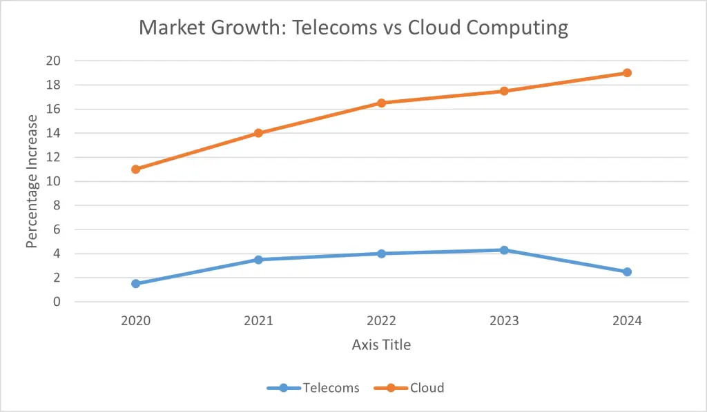
Case Study: Cloud Computing vs U.S. Wireless Telecom
In the 2010s, global cloud computing and U.S. wireless telecom offered two sharply contrasting growth environments that illustrate the economic difference between market expansion and competition for market share.
Cloud Computing: Growth from a Rising Tide
Public cloud infrastructure, led by Amazon Web Services, Microsoft Azure, and Google Cloud, grew rapidly because the entire market was expanding. Corporations were shifting workloads away from on-premise servers toward outsourced data centers. This was not a zero-sum change. Every year, more data, applications, and business processes migrated to the cloud, driven by cost savings, scalability, and the rise of digital services.
This market expansion allowed several firms to grow simultaneously. Together, AWS, Azure and Google Cloud who collectively capture 66% of global cloud infrastructure spending, enjoyed 29% year-on-year growth in Q3 2025.
Many customers adopted multi-cloud strategies, further reducing head-to-head competition. Importantly, pricing remained relatively rational. While discounts existed, no provider had to destroy industry economics to grow, because new demand kept entering the system.
Capital investment was enormous, e.g. data centers, chips, networking, etc. but returns were also strong. Cloud providers could earn high ROIC because they were building into a fast-growing, structurally expanding market rather than fighting over a fixed pie.
U.S. Wireless Telecom: Growth from Taking Share
By contrast, U.S. wireless telecom, dominated by Verizon, AT&T, and T-Mobile, faced a stagnant market. By the early 2010s, smartphone penetration was already high (at 50% of all mobile subscribers by early 2012). Nearly everyone who wanted mobile service already had it. Total industry subscribers grew slowly, if at all.
In that environment, revenue growth had to come from poaching customers. When T-Mobile launched aggressive “Un-carrier” pricing plans, Verizon and AT&T had to respond with promotions, subsidies, and lower margins to prevent defections. Every gain for one carrier implied a loss for another. Customer acquisition became expensive, churn increased, and pricing power eroded.
Even though data usage exploded, competitive intensity meant that much of the economic value was competed away. Carriers invested heavily in spectrum and 5G networks, but returns were constrained because rivalry forced prices down. The market’s lack of expansion converted innovation into a defensive arms race rather than a profit engine.
Why This Distinction Matters
Cloud computing shows how market expansion enables multiple firms to grow with healthy economics. Wireless telecom shows how low-growth markets turn revenue growth into a competitive battleground. In valuation, these environments produce radically different outcomes, even if reported revenue growth initially looks similar. Growth driven by market expansion compounds value; growth driven by share fights often destroys it.
Case Study: The Rise of T-Mobile
A real-world example of the “double-digit growth to single-digit slowdown” pattern can be seen in T-Mobile’s U.S. business over the past decade.
In the mid-2010s, T-Mobile was in a rapid expansion phase. After its turnaround strategy (“Un-carrier”) and the earlier MetroPCS integration, the company began taking meaningful market share from Verizon and AT&T. This culminated in Q2 2014, when T-Mobile reported total revenue growth of about 15.4% year-over-year.
Subscriber additions were strong, churn was falling, and the company was benefiting from both a low base and aggressive pricing and marketing. At that stage, growth was driven by structural changes: customers were switching en masse, network quality was improving, and T-Mobile was still scaling up from a much smaller footprint than its two largest rivals.
Fast-forward a decade, and the growth profile looks very different. By the mid-2020s, T-Mobile had become one of the largest wireless carriers in the U.S. by subscribers following the Sprint merger; in addition, the market itself had matured.
Thus by 2024–2025, T-Mobile’s service revenue growth had slowed to the mid-single digits, with overall revenue growth running around 6–7% year-over-year. The company was still growing, but no longer at the pace seen during its disruptive expansion phase.
4. Reinvestment and Business Model Reality: The Capital Beneath the Growth
4.1 Why Reinvestment Is a Qualitative Question
Reinvestment is often treated as a mechanical output of a model rather than by economic reasoning about how the business actually operates. Capital expenditures may be estimated as a percentage of revenue; working capital as a fixed ratio. But in reality reinvestment is a qualitative expression of the business model itself. How much capital a company must reinvest is determined by asset intensity, operating leverage, the need to maintain existing capacity, and the desired growth.
Asset-intensive businesses, such as manufacturing, logistics, and infrastructure, require continual capital just to stand still. The write-off for depreciation is just a book entry. It is not a measure of the true economic fall in value of the fixed assets. Thus, spending on maintenance may exceed the depreciation charge.
Operating leverage compounds the issue. Businesses with high fixed costs may show attractive margins at scale, but sustaining that scale often requires ongoing investment in capacity, systems, or redundancy.
Reinvestment also reflects management’s tolerance for dilution or leverage. Growth can be financed internally, through equity issuance, or through debt. Each choice has its consequences. A business that avoids dilution may accept higher leverage and balance-sheet risk. One that avoids leverage may dilute shareholders or slow growth.
The key insight is to recognize that reinvestment is rarely optional. Most businesses must reinvest simply to preserve their competitive position. Free cash flow, therefore, is often a lagging indicator of business quality rather than a leading one. Periods of high reported free cash flow can coincide with underinvestment, while low cash flow may be a precursor to growth.
4.2 Hidden Reinvestment Channels
Models often understate reinvestment by overlooking less visible channels. Working capital creep is a common example. As revenue grows, inventories, receivables, and service obligations tend to grow with it, absorbing cash even when margins are stable. Small percentage changes compound meaningfully at scale.
Another frequent blind spot is the misclassification of spending on maintenance as spending to achieve growth. Investments in technology upgrades, store remodels, compliance systems, or customer-facing platforms are often presented as spending to achieve growth even when they are actually the cost of not falling behind. Treating these outlays as spending to achieve growth makes them appear optional and inflates free cash flow. By pretending required reinvestment is discretionary, the model is counting money the business must spend as if it were available to shareholders.
CAPEX includes both spending on maintenance required to sustain the existing business and spending intended to achieve growth but accounting does not distinguish between the two.
Acquisitions are a third channel. Some businesses rely on M&A as a substitute for organic reinvestment, particularly when internal growth opportunities are limited. While acquisitions may appear episodic, in practice they can represent a recurring capital requirement with its own return profile and integration risk.
4.3 Illustrative Example: Growth Constrained by Capital Reality
Consider a business modeled to grow revenues at a steady mid-single-digit rate with modest capital expenditures based on historical averages. Qualitative analysis, however, reveals that recent growth has been supported by aging assets, deferred maintenance, and rising customer service strain. To sustain even the modeled growth rate, the company must invest materially more in systems, capacity, and working capital than the model assumes.
Reconciling this reality forces an adjustment. Either reinvestment must rise, reducing free cash flow and returns (ROIC), or growth expectations must fall. The discipline is not choosing the more attractive outcome, but ensuring that growth, reinvestment, and returns remain internally consistent. This logic follows directly from the principles established in Part I: models do not create economics; they must reflect them.
Case Study: Starbucks and the Illusion of Capital-Light Growth
For much of the 2010s, Starbucks was viewed as a model consumer-brand compounder. Revenues grew steadily, margins were strong, and free cash flow appeared abundant. To many investors, Starbucks looked like a capital-light business, with a global brand, a loyal customer base, and a scalable retail footprint. CAPEX tracked depreciation reasonably closely, and working-capital ratios appeared stable. On paper, growth looked cheap. But the economics beneath that surface were far more demanding.
Starbucks does not just sell coffee; it offers convenience and an experience. These require physical systems. Every store depends on layout design, barista training, digital order flow, equipment reliability, and labor availability. As mobile ordering and delivery grew, Starbucks’ legacy store formats, built for in-store queues, became bottlenecks. In addition, drink complexity increased. Pickup volumes surged. Service times lengthened. Yet much of the investment required to adapt, such as store remodels, equipment upgrades, new pickup formats, and digital integration, was treated as routine maintenance.
By the late 2010s, Starbucks was already relying on deferred reinvestment to keep free cash flow high. Remodel cycles lengthened. Staffing levels were stretched. Technology upgrades lagged volume growth. These decisions flattered reported economics but weakened operational resilience. But a day of reckoning arrived post-COVID.
When customer traffic rebounded in 2021–2022, Starbucks’ stores were unprepared. Drive-thru lanes clogged. Mobile orders and food-delivery orders overwhelmed in-store workflows. Baristas faced rising drink complexity and aging equipment. There was inadequate staffing. Service times worsened, error rates increased, and customer frustration grew. At the same time, employee turnover surged as workloads intensified and wages failed to keep pace. Starbucks was forced into emergency wage increases, retraining programs, and accelerated capital spending just to stabilize operations.
Working capital also crept upward. Digital payments, loyalty programs, inventory breadth, and supply-chain buffers absorbed more cash as the system grew more complex. Meanwhile, international expansion required corporate capital long before local profits emerged.
Management now faced the reality that growth was not free. Starbucks could continue reporting attractive free cash flow by limiting reinvestment, but that meant accepting declining service quality, rising employee attrition, and brand erosion. Or it could reinvest aggressively in labor, store formats, technology, and supply chains, reducing near-term free cash flow to preserve the franchise. It chose the latter. CAPEX rose. Free Cash Flow fell. Margins narrowed.
Starbucks (FY2018–FY2022): FCF, CAPEX, and CAPEX as % of NOPAT
Year
FCF ($m)
CAPEX ($m)
NOPAT est. ($m)
CAPEX as % of NOPAT
2018
9,961.4
1,976.4
3,035.4
65.1
2019
3,240.4
1,806.6
3,282.1
55.0
2020
114.2
1,483.6
1,240.2
119.6
2021
4,519.1
1,470.0
3,820.2
38.5
2022
2,556.0
1,841.3
3,582.8
51.4
From 2018 to 2022, Starbucks’ cash flows show a business that is far more capital-intensive than it appears from earnings alone. In 2018–2019, Starbucks generated solid free cash flow, but even in those good years more than half of after-tax operating profit was consumed by CAPEX. The business required constant reinvestment just to sustain growth and quality. In 2020, that reality became unavoidable. Operating cash flow collapsed while CAPEX barely fell, so reinvestment exceeded NOPAT. Starbucks was forced to fund CAPEX by borrowing. In 2021, profits and cash flow rebounded, temporarily restoring breathing room. But in 2022, higher capital spending and weaker cash generation pushed the reinvestment burden back up again. The pattern is consistent: Starbucks is not a capital-light consumer brand. It is a capital-heavy operating system whose profits are structurally taxed by reinvestment.
The lesson to be learnt is that reinvestment is not a percentage of revenue; it is the cost of staying in the game. Starbucks’ growth had always been capital-hungry. The spreadsheet simply hid it, until the business could no longer.
5. Margins and Competitive Behavior: What Prevents Reversion?
5.1 Structural vs. Cyclical Margin Drivers
Operating margins are among the most tempting variables to extrapolate, and among the most likely to disappoint. The default tendency in competitive markets is toward margin reversion, driven by entry, imitation, customer pressure, and political scrutiny. Understanding what prevents that reversion is therefore a qualitative exercise that should be grounded in industry structure rather than trend analysis.
Several factors deserve scrutiny. Industry concentration matters because fragmented markets typically compete away excess profits, while concentrated industries may sustain rational pricing, though only if coordination is implicit and stable. Customer bargaining power is equally important. Large, price-sensitive customers with alternative suppliers exert downward pressure on margins over time, particularly as those suppliers scale and become more visible. Cost structure also plays a role. Businesses with high fixed costs may experience sharp margin expansion during upcycles, but those gains often retreat when volumes normalize.
Regulatory and political visibility acts as a final constraint. High margins in essential services, such as infrastructure, healthcare, or consumer-facing platforms, tend to attract scrutiny. Even in the absence of formal regulation, public and political pressure can cap pricing power or impose additional compliance costs. These forces explain why margins tend to revert: elevated profitability attracts new entrants. Margins that are sustained or widening therefore require structural justification, not just favorable conditions.
5.2 When Margin Expansion Is Plausible, and When It Isn’t
Margin expansion is most plausible when driven by operating leverage that reflects genuine fixed-cost absorption within a defensible competitive position. For example, software platforms with high upfront development costs and low marginal costs can expand margins as revenue rises, provided switching costs and differentiation limit competitive erosion.
By contrast, margin gains driven solely by scale without defensible differentiation are fragile. Cost efficiencies can often be replicated. Suppliers’ contracts can be renegotiated. Customers may demand concessions. Competitors invest to match capabilities. In these cases, operating leverage may improve margins temporarily, but competitive dynamics usually reassert themselves.
The distinction is subtle but critical. Operating leverage explains how margins can expand; competitive advantage explains why they might stay expanded. Models that assume both without examining their interaction risk embedding optimism where evidence is weakest.
5.3 Illustrative Example: Margins That Peak Before the Model Does
Consider a business reporting steady margin expansion driven by price increases and cost rationalization. Management guidance extrapolates these gains, and the model reflects continued improvement. A qualitative review, however, reveals rising customer churn, aggressive competitor pricing, and growing regulatory attention as profitability increases.
In this setting, current margins may represent a local peak rather than a new equilibrium. Competitive responses lag reported results, and regulatory processes move slowly, but both are building. A disciplined analyst would cap margins at a level supported by industry economics or explicitly fade them over time, even if near-term momentum remains strong.
This adjustment is not pessimism; it is a more realistic perspective. The purpose of the model is not to reward recent success, but to test whether that success can persist. As was discussed in Part I, margins are outcomes of structure and behavior, not ratios to be assumed.
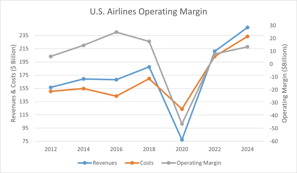
Case Study: U.S. Airlines and the Gravity of Margin Reversion
In the mid-2000s, U.S. airlines looked like a textbook case of an industry finally escaping its own history. After decades of value destruction, a wave of bankruptcies and mergers, notably Delta with Northwest, United with Continental, and American with US Airways, left the industry far more consolidated. Capacity discipline improved, planes flew fuller, and operating margins rose into the low-to-mid teens, levels that would once have seemed impossible.
Data Source: Bureau of Transportation Statistics
But those margins immediately attracted pressure. Low-cost carriers such as Southwest, Spirit, and Frontier expanded aggressively, copying network economics on profitable routes while avoiding the legacy cost base. New aircraft technology allowed point-to-point competitors to cherry-pick routes that had once been protected by hub dominance. At the same time, customers became more price-sensitive as online booking platforms made fares fully transparent. Airlines could no longer quietly raise prices; any increase was instantly visible and matched or undercut by rivals.
Political pressure added another layer. As profitability returned, airlines became a visible target for regulators and consumer advocates. Fees, route cuts, and pricing practices drew scrutiny, limiting how far airlines could push their advantage even when demand was strong.
All of these forces, such as entry, imitation, customer bargaining power, and political oversight, pulled margins back toward competitive norms. The industry could not simply “lock in” high returns; every period of good profitability set in motion forces that undermined it.
Yet airlines also illustrate why margin reversion is not automatic. The same consolidation that created profits also created structural barriers. Time slot controls at airports like JFK and Heathrow limited new entry from startup airlines. Commercial aircraft manufacturing is effectively a duopoly, constraining how quickly competitors can add capacity. Network effects from hubs, loyalty programs, and corporate contracts made incumbent airlines harder to displace.
As a result, airline margins today are higher and more stable than in the past, but they remain cyclical and fragile. The industry sits in a narrow band between two forces: competitive gravity pulling profits down, and structural frictions holding them up. That tension is the essence of margin reversion in the real world.
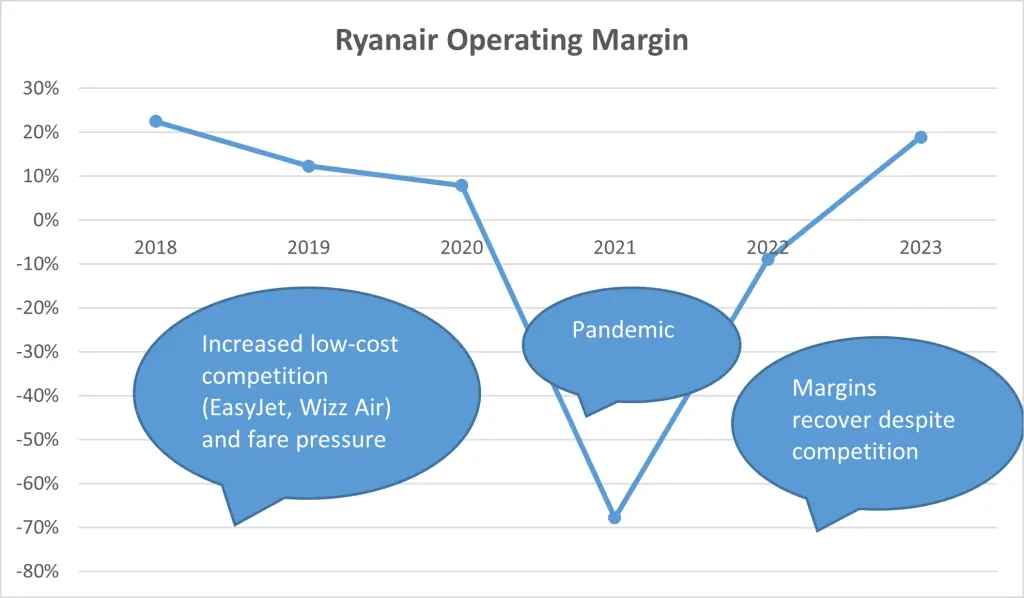
Case Study: Ryanair and the Tug-of-War Between Margin Reversion and Structural Advantage
Ryanair offers a real-world illustration of how competitive forces push margins toward reversion and why, in some cases, they do not fully succeed.
Through the 2000s and 2010s, Ryanair built one of the highest and most stable operating margin profiles in global aviation, often in the 15–25% range. In a textbook competitive market, such margins should have been temporary. And indeed, the classic forces of reversion appeared quickly.
Entry and imitation came first. EasyJet, Wizz Air, and a long line of ultra-low-cost carriers copied Ryanair’s stripped-down service model, dense seating, fast turnarounds, and ancillary-revenue playbook. Aircraft manufacturers made standardized narrow-body jets widely available, lowering capital barriers to entry. Routes that were once Ryanair strongholds saw new competitors match fares within days.
Customer pressure intensified as well. Online aggregators and fare-comparison tools made prices perfectly transparent, turning airline seats into near-commodities. Any attempt to raise ticket prices triggered immediate demand loss. Ryanair’s own passenger growth became increasingly price-elastic, forcing it to pass fuel cost swings through to margins rather than customers.
Political scrutiny added a further drag. Ryanair’s labor practices, airport subsidy arrangements, and aggressive fee structures attracted regulatory attention across the EU. Court rulings on pilot contracts, minimum service rules, and consumer-rights regulations raised costs and limited pricing flexibility, exactly the kind of institutional pressure that compresses excess returns.
Yet Ryanair also shows why margin reversion is not inevitable. Its structural advantages proved unusually durable. It locked in ultra-low unit costs through massive aircraft orders that secured better pricing from Boeing, long-dated airport fee agreements with secondary airports, and a ruthless focus on cost discipline embedded in corporate culture. Its scale created purchasing power advantages smaller rivals could not match. Its brand became synonymous with “lowest fare,” anchoring customer expectations in its favor.
The result is a compromise outcome. Ryanair’s margins have fluctuated and compressed during downturns and cost shocks, but they remain structurally above most European peers. Competitive gravity pulled its profits down; structural frictions held them up.
6. WACC and Risk Perception: Pricing Uncertainty, Not Optimism
6.1 WACC as a Qualitative Risk Assessment
In a buy-side framework, the weighted average cost of capital (WACC) should be understood not as a spreadsheet output, but as a qualitative statement about business risk. While tools such as the Capital Asset Pricing Model (CAPM) can inform the estimate, they cannot substitute for judgment. WACC is meant to price how fragile, uncertain, volatile, or exposed a business’s cash flows truly are, and not to validate an attractive narrative.
Several qualitative drivers shape this assessment. Earnings volatility is the most obvious. Businesses exposed to cyclicality, commodity prices, or discretionary demand warrant higher required returns than those with stable, contractual cash flows. Customer concentration matters as well. A firm reliant on a small number of counterparties may appear stable in good times, yet face abrupt downside if relationships change. Balance-sheet fragility compounds these risks. Leverage magnifies both outcomes and errors, increasing the probability of permanent capital impairment even when near-term earnings look secure.
Regulatory and technological risk are equally important. Industries subject to shifting regulation, political scrutiny, or rapid technological change face uncertainty that rarely shows up in historical betas. These risks are forward-looking and asymmetric. WACC should reflect that asymmetry, even when recent results appear benign.
Beta shows how much a stock tends to rise or fall when the market goes up or down. Historical beta: How volatile the stock is relative to the market in the past. Bottom-up beta: How volatile the stock is expected to be relative to the market in the future.
6.2 Common Misuses of WACC
Despite its conceptual importance, WACC is often misused. One common error is lowering WACC to “make the valuation work.” When the intrinsic value falls short of expectations, adjusting the discount rate becomes a convenient regulating valve. This practice reverses causality: valuation should be a function of risk.
Another mistake is confusing cheap debt with low risk. Low borrowing costs may reflect liquidity conditions, collateral, or central bank policy, not the underlying stability of operating cash flows. A firm can borrow cheaply and still be economically fragile. Treating low interest expense as evidence of safety understates equity risk.
Finally, analysts sometimes adjust WACC mechanically for changes in capital structure, rather than for changes in asset risk. Increasing leverage may lower the weighted average mathematically, but it does not reduce business risk. In many cases, it increases it. WACC should be anchored to the risk of the operating assets, not the financing mix layered on top.
6.3 Illustrative Example: When the Right WACC Feels Uncomfortable
Consider a business with steady recent earnings, modest leverage, and a history of meeting guidance. On the surface, it appears stable. A qualitative review, however, reveals customer concentration, exposure to a single regulatory regime, and sensitivity to technological substitution. None of these risks have materialized recently, but all are plausible.
Applying a higher WACC to reflect these uncertainties often feels uncomfortable because it materially reduces valuation. Sensitivity analysis may reveal that most of the upside depends on assuming away these risks. That discomfort is instructive. It highlights where the investment case relies less on economics and more on optimism. As emphasized in Part I, WACC is not a plug; it is a discipline that forces honesty about the risks being underwritten.
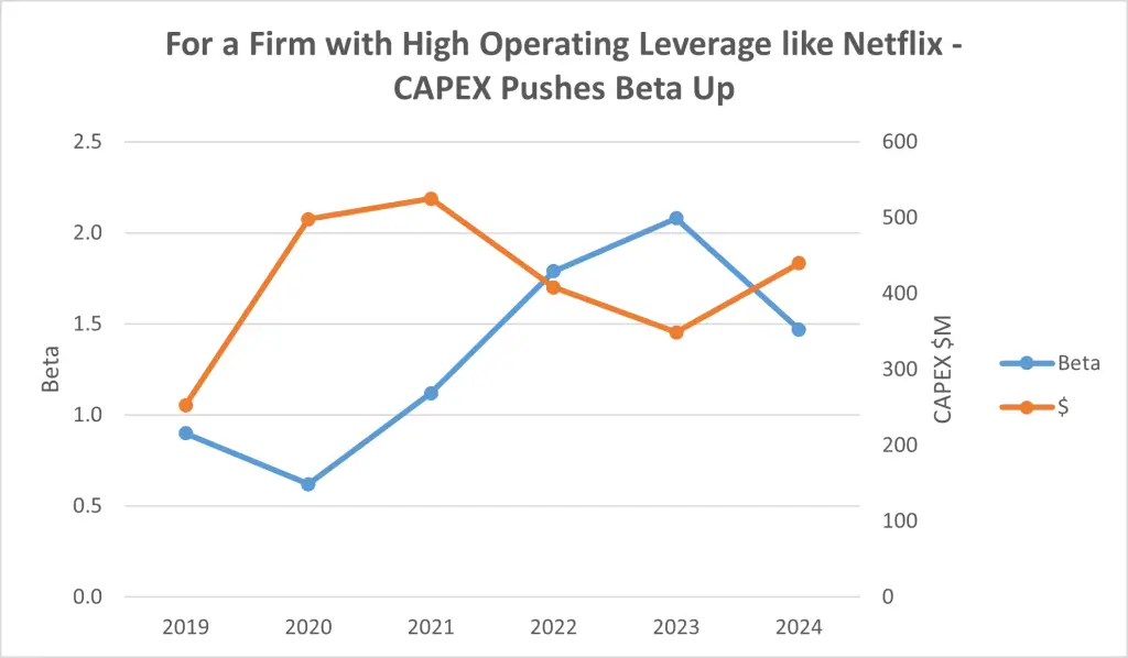
Case Study: Netflix and the Illusion of a “Stable” Beta
In 2017, Netflix appeared to be entering a new phase of its corporate life. The company had upended the physical movie rental business, surpassed 100 million subscribers globally, was exhibiting strong revenue growth, and was increasingly being described as a “media platform” rather than a speculative technology company. Its stock had appreciated sharply, and measured volatility had declined. As a result, Netflix’s trailing five-year beta fell to around 1.0, roughly in line with the market.
Many analysts took this at face value. Plugging the lower beta into CAPM, they concluded that Netflix’s cost of equity had fallen materially. With a lower discount rate, discounted cash-flow models showed significantly higher valuations. In this framework, Netflix appeared to have “matured” into a safer business. But this conclusion rested on a mistake: it confused stock price behavior with business risk.
A forward-looking analysis of Netflix’s economics told a very different story. By 2017–2018, Netflix was no longer competing against fragmented cable networks or DVD distributors. It was competing against Disney, Amazon, Apple, Sony, HBO, and eventually dozens of well-funded global streaming services. The market structure was shifting toward content arms races, where differentiation depended on spending more, not less. Barriers to entry in distribution were falling, not rising. Customer switching costs were modest, and the resulting streaming service churn was painful. Critically, Netflix’s business model was structurally dependent on licensed content. When the major studios began raising licensing fees and pulling their most valuable titles back for their own streaming platforms, Netflix found itself exposed. It was forced into massive, recurring investment in original programming simply to maintain its existing value proposition.
From a business-risk perspective, Netflix was becoming more fragile, not less. Cash-flow volatility was rising. Margins were dependent on subscriber growth continuing indefinitely. Competitive intensity was increasing. Political scrutiny over content, pricing, and market dominance was growing.
A disciplined analyst would therefore have concluded that Netflix’s asset risk was rising, not falling. That implied a higher forward beta, perhaps 1.5 or more, reflecting greater cyclicality, competitive pressure, and uncertainty over long-term profitability.
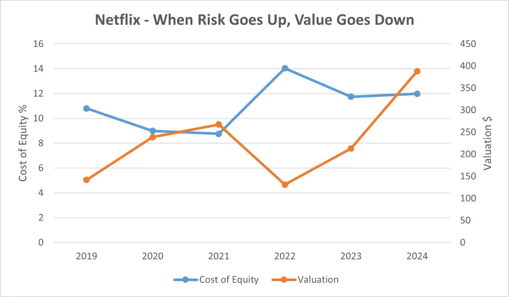
Using the trailing beta of 1.0 or less implicitly treated Netflix as a diversified consumer platform with stable economics. Using a forward-looking beta of 1.5 or more treated it as what it actually was: a highly competitive, capital-hungry media business exposed to escalating rivalry and uncertain pricing power. (See chart)
The difference is decisive. A 300-basis-point increase in cost of equity could reduce Netflix’s intrinsic value by 25–30% in a DCF model. When growth slowed and competition intensified in the years that followed, the market ultimately repriced the stock accordingly.
The lesson is not that Netflix was a bad company. It is that WACC must reflect the future economic reality of the business, not the recent calm of its stock price. Backward-looking betas describe the past. Valuation requires judgment about the risks that lie ahead.
7. Terminal Assumptions and Economic Gravity: Where Belief Is Tested
7.1 Terminal Value as a Concentration of Assumptions
Terminal value is where a valuation model expresses its strongest convictions, but it is also where supporting evidence is often weakest. By construction, the terminal period accounts for a disproportionate share of intrinsic value, particularly for long-duration businesses. Small changes to terminal growth rates, steady-state margins, or long-run returns on capital can overwhelm years of explicit forecasting.
Because evidence thins as horizons extend, terminal value must be anchored to qualitative realities rather than extrapolated trends. Long-term industry structure matters: fragmented industries tend to normalize returns faster than concentrated ones; capital-light sectors invite entry more readily than asset-specific ones. Capital inflows are a persistent force. High returns attract competitors, private capital, and substitutes, all of which pressure margins and reinvestment returns over time. Regulatory normalization is another anchor: periods of permissive oversight or favorable rules rarely persist indefinitely. Finally, economic growth ceilings impose limits: companies cannot outgrow their markets. Terminal value, then, is not so much a forecast but an economic hypothesis of the future.
7.2 Normalcy vs. Exceptionality
The default outcome in competitive markets is reversion toward normalcy. Excess returns attract competition, and competition reduces returns. Even “great businesses” face economic gravity over time through imitation, customer bargaining, regulatory scrutiny, or capital deepening that lowers incremental returns. This does not imply mediocrity. It implies that stability is more defensible than perpetual improvement.
Exceptions exist, but they are rare and must be justified by reference to business structure. Durable network effects, regulatory monopolies, or platforms with extreme switching costs may sustain returns above the cost of capital for extended periods. Even then, the burden of proof rises as assumptions extend further into the future. When terminal models assume indefinite excess returns without specifying why capital cannot enter, why customers cannot switch, or why regulation cannot intervene, the assumption shifts from analysis to conjecture. The objective should be to distinguish between actual exceptionality, supported by structure, and assumed exceptionality, supported primarily by continuing the trend.
7.3 Illustrative Example: A Terminal Value That Carries the Case
Consider a business whose explicit forecast delivers modest free cash flow growth, while the terminal value contributes the majority of estimated intrinsic value. The terminal case assumes sustained high ROIC, stable margins, and growth modestly above GDP. On paper, these inputs appear conservative. But qualitative factors may tell a different story. The industry is experiencing capital inflow, customer bargaining power is rising, and regulatory attention is increasing as profitability becomes more visible.
This may be remedied by fading terminal ROIC toward industry norms, trimming terminal growth to reflect market maturity, or modestly rising WACC, all of which will reduce valuation. Such an exercise shows that the investment thesis depends a great deal on long-run immunity to competition. This terminal discipline protects against narrative drift. And forces the model to respect economic reality, consistent with the guardrails established in Part I.
Case Study
Visa and the Long Fade of Network Economics
Visa is often presented as the archetype of a “terminal compounder.” Its business model is capital-light, its brand is global, and its network effects are formidable. For much of the past two decades, Visa has earned extraordinary returns on invested capital, often above 30%, as digital payments displaced cash and the company scaled a toll-booth model across an expanding volume of transactions. In a standard valuation model, it is tempting to assume that these economic factors simply persist. Yet Visa also illustrates why terminal value must reflect economic reality, and not historical success.
In the explicit forecast period, Visa’s growth is easy to justify. Electronic payments continue to take share from cash, e-commerce expands, and global travel recovers. Margins remain high because incremental transaction volume flows through a largely fixed cost base. ROIC stays elevated because little new capital is required to process more payments. These assumptions are grounded in observable trends. The difficulty begins when those trends are projected indefinitely.
Visa’s industry is not closed. Its very profitability attracts capital and innovation. Fintech firms, real-time payment systems, buy-now-pay-later platforms, and even central bank digital currencies all represent alternative rails for moving money. Merchants, increasingly aware of the fees embedded in card payments, are more willing to steer customers toward cheaper methods. Regulators in Europe, India, and Australia have already imposed fee caps or routing mandates that reduce returns. None of these forces destroys Visa’s business, but each erodes the incremental economics of growth.
A disciplined terminal model therefore does not assume Visa’s 30%+ ROIC forever. Instead, it allows that ROIC to fade gradually toward a still-attractive, but more normal level (say the mid-teens) as competition, regulation, and capital deepening take effect. Margins remain healthy, but not immune. Growth continues, but closer to global payments growth rather than a perpetual premium to GDP.
This distinction matters because Visa’s valuation, like many high-quality compounders, is dominated by its terminal value. If the model assumes a flat, permanent excess return, the terminal block silently carries the entire investment case. If instead ROIC is allowed to decay slowly, the valuation still supports a strong business, but offers a more realistic perspective. The terminal question is not whether Visa stays good, but whether it stays unassailably great. Letting ROIC fade toward a defensible steady state respects both Visa’s structure and the competitive forces that inevitably surround it.
Case Study: IBM (2000s–2010s): Why Rising Business Risk Forces Terminal Assumption Discipline
For much of the early 2000s, IBM looked like a model compounder. It had transformed itself from a hardware manufacturer into a high-margin enterprise services and software company. Switching costs were high, customer relationships were sticky, and ROIC consistently exceeded the cost of capital. For a time, it was reasonable to believe that IBM could sustain supernormal economics indefinitely.
But beneath that surface stability, the economic foundations of the business were quietly weakening, making IBM’s terminal ROIC structurally indefensible. Cloud computing was commoditizing infrastructure. Open-source software was eroding pricing power. As differentiation faded and competition intensified, IBM’s ability to earn excess returns declined. The correct modeling response was not to assume a permanent moat, but to fade ROIC gradually toward industry norms or only a modest premium to WACC.
In addition, IBM’s end markets matured, making long-run growth assumptions increasingly unrealistic. Core segments such as mainframes, on-premises software, and traditional IT services were saturated and in secular decline. Even IBM’s strategic pivots, toward analytics, AI, and later hybrid cloud, were largely defensive, offsetting lost revenue rather than creating new demand. A disciplined valuation therefore required trimming terminal growth below GDP, tightening the reinvestment-growth relationship, and abandoning the idea that a mature incumbent could compound at historical rates.
Moreover, IBM’s business risk rose structurally over time, justifying a higher, not lower, terminal discount rate. Customer switching costs fell. Technological disruption accelerated. Competitive intensity increased. These forces made IBM’s future cash flows more sensitive to the business environment. In valuation terms, that means a modestly higher WACC (or at minimum, refusing to let beta drift downward) is warranted.
IBM illustrates a core valuation principle: when industry structure weakens and competitive pressure intensifies, conservatism in terminal assumptions is not pessimism; it is realism. Fading ROIC, trimming growth, and modestly raising WACC are not optional tweaks; they are necessary corrections to avoid structurally overstating long-term value.
8. Synthesis: Using the Model as a Judgment Filter, Not a Forecast
The purpose of Part II has been to show that the key inputs in a quantitative equity model are not independent variables, but expressions of the business environment. ROIC, growth, reinvestment, margins, WACC, and terminal assumptions are different perspectives on the same business. Weakness in one qualitative area rarely remains isolated. It tends to surface across multiple metrics, often in subtle but reinforcing ways.
For example, fragile competitive positioning does not only threaten margins; it usually shows up as declining forward ROIC, higher reinvestment requirements to defend share, and greater earnings volatility that should be reflected in WACC.
Similarly, aggressive growth assumptions often collide with reinvestment reality. If growth is modeled as rapid but capital-light, the inconsistency will eventually appear, either through implausibly rising ROIC, overstated free cash flow, or heroic terminal assumptions. These tensions are not modeling errors; they are analytical signals.
This is why cross-checks matter more than precision. Growth must reconcile with reinvestment. Reinvestment must reconcile with ROIC. ROIC must reconcile with competitive structure. Margins must reconcile with customer power and cost rigidity. WACC must reconcile with qualitative risk. Terminal value must reconcile with economic gravity. When these relationships cohere, the model gains explanatory power. When they do not, the model is revealing where assumptions conflict, optimism concentrates, or further work is required.
The practical takeaway is straightforward. The model’s value does not lie in forecasting outcomes or producing a single “correct” valuation. It lies in exposing where belief is concentrated and where error would be most costly. Sensitivity analysis is useful not because it produces ranges, but because it identifies which assumptions dominate results. Almost invariably, the highest-risk assumptions are also the least discussed. These tend to be forward ROIC, reinvestment intensity, margin durability, and terminal behavior.
Used properly, the model becomes a method of validation. It disciplines intuition, surfaces hidden bets, and forces qualitative reasoning to confront quantitative consequences.
As emphasized throughout Part I, the goal is not to eliminate uncertainty, but to understand precisely where it resides, and to price it honestly.
9. Closing: From Spreadsheet Confidence to Analytical Caution
Part I of this article suggested a framework for analysis. It set out the basic economic variables, ROIC, growth, reinvestment, margins, WACC, and terminal assumptions, and showed how they interact within a quantitative equity model. That framework is essential. Without it, analysis risks becoming narrative-driven, impressionistic, or inconsistent.
Part II serves a different purpose. It invokes critical thinking. Each section has emphasized that the most important inputs in a model are not mechanical outputs but stem from qualitative judgments about competition, capital, risk, and durability. These judgments are uncertain by nature and prone to overconfidence precisely because they sit behind clean numbers. The role of the analyst is not to eliminate that uncertainty, but to confront it honestly.
Good models do not predict outcomes. What they can do, when used properly, is clarify what must go right for an investment to work. They make explicit the assumptions about growth persistence, reinvestment efficiency, margin durability, and risk tolerance that are otherwise left implicit.
Just as importantly, good models show what happens when things do not go right. They reveal how sensitive value is to fading returns, higher capital intensity, competitive response, or a more honest cost of capital. This asymmetry is critical. Most investment mistakes are not caused by minor forecasting errors, but by underestimating downside paths that were visible but insufficiently weighted.
The transition from spreadsheet confidence to analytical caution is therefore not a retreat from rigor; it is objective. A model that produces precise answers without discomfort is usually missing something. A model that provokes unease, because small changes have large effects, or because assumptions are hard to defend, is doing its job.
In a buy-side context, the highest compliment a model can earn is that it sharpens judgment. It should narrow the field of plausible outcomes, identify where capital is truly at risk, and help the investor decide whether the uncertainty being underwritten is worth the price. That, ultimately, is the discipline Part I sought to build and Part II has sought to preserve.